|
Automated optical digital linearity deviation meter
Korolev А.N., Lukin A.Ya., Polishchuk G.S.
Measurement of deviations from linearity, flatness and alignment is the
important aspect of technologies, relating to mechanical engineering, aircraft industry
and shipbuilding. Besides, said measurement is widely used while controlling
the quality of plates, guiding elements of machines, frames of engines of large
dimensions, rolling mills, presses and turbines. Moreover, this type of
measurement is used to check linearity of moving of parts of machines as well
as of other mechanisms.
The Alignment Monitoring System, in which
automatic reflectivity design [1] is implemented, is known. If we apply this
system, the limiting value of allowable root-mean-square deviation (“RMS
deviation” below), relating to a random component of the basic error does not
exceed 0.05 mm at any distance up to 10 m.
Besides, Laser Linearity Deviation Meter
[2] has been developed. The basic feature of this meter is that it includes
axicon, used for forming the laser beam ring structure, which is convenient
when making measurements. Measurement of co-ordinates is performed by taking
into account position of the ring structure central spot, diameter of which is
some times less than the diameter of the laser beam. Measurement error is
determined by the accuracy of measurement of the central spot co-ordinates at
the speckle-sound background. Value of error may be determined by using the
formula ± (0,004 + 3·10 – 3 L), where L
is the distance in meters.
Another device, used for measurement of
deviations, is known under the name “PPS-11 Measuring Sighting Telescope”. This
device is intended to measure linearity deviations, relating to long objects,
as well as to measure alignment deviations, relating both to holes and tubes.
Moreover, said device is used for performing evaluation of non-parallelism,
extent of absence of perpendicularity and deviation from horizontal position,
which relate to surfaces of various articles. “LOMO” PLC was engaged in
manufacturing this optical instrument some years ago, and at present said
instrument is widely used at the mechanical engineering, machine-tool building
and shipbuilding plants for carrying out accurate measurements of linearity
deviations.
Such instruments, which are known under the
name “Alignment Telescopes”, are manufactured by some companies of other
countries. For example, optical devices, produced by the “Taylor Hobson”
company of Great Britain [5], have a very high reputation.
An alignment telescope includes objective
lens and focusing lens, which are employed to form image of a measuring mark in
the plane of cross hairs. Said measuring mark may be located at any of the
distances, lying within the range 0 – 30 meters, from the telescope end face.
It is assured that whenever the focusing lens is moved in longitudinal
direction it is moving along the guiding line without any deviations. In this
way the required position of the sighting line with respect to the optical axis
of the system, including objective lens and focusing lens, is maintained. Value
of misalignment of the optical mark image with respect to the sighting line is
measured by means of the optical micrometer, which includes tilting
plane-parallel plate and measuring drums. Position of these drums is changing
while the plane-parallel plate is being turned around two mutually
perpendicular axes. Operator monitors alignment by viewing image in the device
ocular.
When performing measurements an operator
should bring an image of the measuring mark into focus within the alignment
telescope. To achieve focusing an operator must move focusing lens by using
special control handle. Then misalignment of the measuring mark image with
respect to the sighting line is subject to measurement. This measurement is
performed by way of turning the plane-parallel plate around the horizontal axis
and the vertical axis as well as by bringing the mark image centre and the
cross hairs centre into perfect coincidence. It should be noted that quantity
of measurements depends upon the distance between the measuring mark and the
telescope end face. If said distance exceeds 10 meters then measurement should
be carried out not less than 10 times.
The main disadvantages of such optical instruments
are insufficient accuracy of measurements and low productivity of an operator’s
labour, that is caused by great number of operations, performed manually.
The digital device of OPTRO-PPS-031 type
[6], intended to measure linearity deviations by means of sighting the
measuring mark, was developed. Said meter includes the digital TV-camera, which
functions as a photo-detector. Both processing of data bulk, relating to
TV-images, and controlling all the procedures of measurement are performed by way
of using the corresponding software.
In the digital device, presented here, the
function of a photo-detector is carried out by the BR-1340LM-UF type digital
TV-camera (www.es-experts.ru). This camera includes the
CCD-matrix of dimension 5,7 mm x 6,3 mm (number of pixels is 1280 x 1024, the
pixel size is 5,2 micron x 5,2 micron).
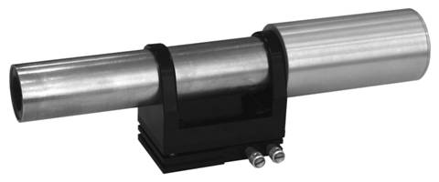
In Fig.1 the side view of the digital meter
alignment telescope and the shape of the measuring mark are shown.
Fig. 1

The measuring mark is a transparent
element, on the surface of which circles of various diameters, relating to a
single centre, are drawn. This mark is illuminated by means of a light diode
matrix. The software database employs the table, which includes such data as circle
consecutive numbers, circle diameters and relative width of rings, located
between adjacent circles. Values of the circle diameters are presented by a
functional, which allows both to calculate some values of relative width of
rings and to apply these values for automatic determining a circle consecutive
number. The measuring mark shape affords an opportunity for carrying out
measurements within the range 0 – 30 meters. If distance is short then
measurement is performed by way of using image of the central circles of small
diameters. If distance is long image of the circles of small diameters may not
be formed, and that is why measurement is performed by way of using image of
the circles of large diameters.
Applying the measuring mark of the maximum
diameter 90 mm affords the opportunity for performing measurements at the
distance 30 meters. Provided the diameters of the mark peripheral circles are
large enough the distances, at which measurements are performed, may be as long
as 50 or even 100 meters. The most important limiting factors in this case are
stiffness of a measuring stand and environment stability.
Block diagram of the digital device, which
is used to measure both the linearity deviations and the alignment deviations,
is shown in Fig. 2. This diagram includes the following elements: measuring
mark 1, provided with illuminator; object, such as frame, plate, slab, guiding
element etc., subject to measurement; the main objective lens 3; the focusing
lens 4; optical system 5, which forms an inverted image; digital TV-camera 6;
control block 7; computer 8, to which TV-camera 6 and control block 7 are
connected. The block 7 controls functioning of the drive, which provides
step-by-step movement of the focusing lens 4. The term “drive, providing
step-by-step movement” means aggregation of a step-by-step engine and a
mechanism, which are employed to convert rotational movement of said engine
into the focusing lens translation.
Fig. 2
When the process of measurements is being
carried out the measuring mark images are located in different positions on a
surface of an object under study. These positions correspond to the route,
along which measurements should be performed, and they are located at various
distances from the deviation meter.
Focusing of the lens 4 at the measuring
mark image is carried out after the computer generates the corresponding
command, that leads to movement of said lens. While the focusing lens is moving
each of the frames, formed by the TV-camera, is used to calculate the focusing
parameter. Value of this parameter is determined by the sum of the first
derivative magnitudes, relating to all points of a 2-D array, used to display
the measuring mark. The process of automatic focusing is completed at the
moment the maximum value of the focusing parameter is obtained.
As a result of performing the above
mentioned process values of both the focal distance and the image scale are
subject to change.
According to the software, employed to
carry out measurements, the following procedures, relating to each of the
measuring mark positions, are performed:
a) automatic throwing the measuring mark
image into focus with respect to the TV-camera matrix surface;
b) determining an image scale or, to be
exact, the optical system magnification (by way of measuring the diameters of
circles, by comparing the measured values with their nominal values and by
calculating the weighted mean value);
c) establishing the value of distance to
the measuring mark (by way of using the tabulated database, which refers image
scale to determined distance);
d) ascertaining position of the measuring
mark image centre on the matrix surface (by way of measuring the image centre
co-ordinates with respect to each of the circles as well as by determining the
weighted mean value with respect to the circles, subject to examination);
e) calculating the value of misalignment of
the measuring mark image centre in relation to co-ordinates of the sighting
line trace;
f) calculating the value of misalignment of
the measuring mark centre in the object space with respect to the base-line.
The term “sighting line trace” means the
point where the sighting line intersects the plane of the TV-camera light
sensitive matrix.
Performing each of the abovementioned
procedures is based on digital processing of the measuring mark image, formed
on the matrix surface. It should be noted that the digital processing methods
offer averaging different results of a measurement. Specifically, the following
results may be subject to averaging:
1) the results of a measurement of
the centre co-ordinates for each of the frames, formed by the TV-camera (this
averaging relates to those circles, which are displayed due to imaging the
measuring mark);
2) the results of a single
measurement conformably to predetermined number of frames;
3) the results of a measurement
conformably to predetermined number of single measurements;
4) the results of measurements
in conformity with the predetermined number of focusing positions.
Applying digital processing methods allows
yielding very accurate result of measurements as well as to estimation of value
of a random error, which presents the quality of measurements.
Below the following equation symbols will
be used:
L – distance from the deviation meter to the measuring mark in meters;
X, Y – co-ordinates of the mark image
centre along the axes X and Y in microns according to the scale of co-ordinates
of the light sensitive matrix;
dX, dY – deviation of a component profile
from the base line in microns relative to the co-ordinates X and Y;
V – magnification of an objective lens in relative units.
Let us consider calculation of profile of a
component, subject to measurement, which is carried out by taking into account
linearity deviation from the Y-axis.
Provided the process of measurements yields
the results for N points, located on
the distance scale, the component profile co-ordinates in each of n measurement points (n = 1 … N) should be determined by using the equation
Pn = (Yn– Yc) · Vn , (1)
In
this equation Ycis the
co-ordinate of the sighting line trace within the detecting TV matrix. (The
procedure of determining the co-ordinates of the sighting line trace within the
light sensitive matrix of a TV-camera will be considered below).
The basic purpose of performing the
measurements is to define a component profile relative to base-line, by means
of which the initial point and the final point are located with reference to
the co-ordinates P1 and PN . That is why co-ordinates
of the base line should be determined
 , (2) , (2)
And only then by using the equation (3)
the profile co-ordinates relative to the base line may be determined
dYn = Pn– Bn, (3)
The results of measurements of the rail profile co-ordinates are
included in the table 1 for illustration. The measurements were performed in
the mode, which may be outlined in the following way: bringing the objective
lens into focus (5 times) – carrying out 5 measurements each time the objective
lens is brought into focus – forming 5 frames relative to each of the measurements.
It is obvious that measurement information, used for each of the profile
points, contains 125 frames.
The table 1 includes the following additional equation symbols:
sdX –
average value RMS deviation, relating to dX (in microns);
sdY – average value RMS deviation,
relating to dY (in microns);
sX – average value RMS
deviation, relating to X (in microns);
sY – average value RMS
deviation, relating to Y (in microns);
sV – average value RMS
deviation, relating to V (in relative
units).
Table 1
Results of measurements of the article profile
| n |
L, м |
dX, мкм |
dY, мкм |
sdX, мкм |
sdY, мкм |
X, мкм |
Y, мкм |
sX, мкм |
sY, мкм |
V |
sV |
| 1 |
1.608 |
0 |
0 |
0.3 |
0.3 |
3396.50 |
2357.17 |
0.06 |
0.07 |
3.9406 |
0.0001 |
| 2 |
1.71 |
24.1 |
-71.5 |
1.0 |
0.6 |
3398.76 |
2403.06 |
0.19 |
0.14 |
4.1378 |
0.0001 |
| 3 |
1.813 |
4.4 |
-131.6 |
0.7 |
0.3 |
3390.71 |
2448.32 |
0.16 |
0.06 |
4.335 |
0.0003 |
| 4 |
1.918 |
-15.8 |
-157.3 |
0.5 |
0.4 |
3383.19 |
2497.81 |
0.11 |
0.09 |
4.5312 |
0.0005 |
| 5 |
2.023 |
8.4 |
-158.2 |
0.1 |
0.1 |
3385.70 |
2548.91 |
0.02 |
0.03 |
4.7264 |
0.0002 |
| 6 |
2.13 |
40.8 |
-128.0 |
0.4 |
0.3 |
3389.64 |
2602.85 |
0.08 |
0.07 |
4.9217 |
0.0005 |
| 7 |
2.236 |
59.7 |
-78.0 |
0.2 |
0.3 |
3390.65 |
2656.38 |
0.04 |
0.06 |
5.1144 |
0.0005 |
| 8 |
2.344 |
74.8 |
-25.9 |
0.6 |
0.5 |
3390.84 |
2707.14 |
0.11 |
0.10 |
5.309 |
0.0008 |
| 9 |
2.45 |
67.4 |
36.4 |
0.5 |
0.7 |
3386.99 |
2755.61 |
0.09 |
0.12 |
5.4996 |
0.0003 |
| 10 |
2.558 |
30.0 |
83.6 |
0.4 |
0.4 |
3378.07 |
2798.56 |
0.07 |
0.08 |
5.6919 |
0.0004 |
| 11 |
2.664 |
18.1 |
117.5 |
0.4 |
0.3 |
3374.09 |
2836.31 |
0.07 |
0.04 |
5.8834 |
0.0004 |
| 12 |
2.771 |
-41.0 |
129.0 |
0.5 |
0.4 |
3362.61 |
2867.81 |
0.08 |
0.08 |
6.0739 |
0.0006 |
| 13 |
2.877 |
-23.4 |
128.6 |
0.8 |
1.3 |
3364.07 |
2895.48 |
0.13 |
0.21 |
6.2649 |
0.0002 |
| 14 |
2.982 |
-24.1 |
110.1 |
0.4 |
0.7 |
3362.61 |
2918.40 |
0.07 |
0.11 |
6.4537 |
0.0005 |
| 15 |
3.087 |
-6.0 |
85.4 |
0.4 |
0.4 |
3364.06 |
2939.10 |
0.06 |
0.07 |
6.643 |
0.0002 |
| 16 |
3.193 |
11.0 |
47.3 |
0.8 |
1.2 |
3365.27 |
2957.00 |
0.12 |
0.19 |
6.8344 |
0.0006 |
| 17 |
3.299 |
0 |
0 |
0.4 |
1.0 |
3362.43 |
2972.36 |
0.06 |
0.14 |
7.0235 |
0.0006 |
The results,
presented in the Table 1, indicate that the average value RMS deviation,
relating to co-ordinates (sX, sY) of
the measuring mark image centre, does not exceed 0.2 microns. When the distance
is changed within the range 1.6 – 3.3 m the average value RMS deviation,
relating to the results of measurements (sdX,
sdY), does not exceed 1.5 microns. If we consider the value sV, presented in the Table 1, it becomes
obvious that the value of error, which takes place when distance L to the
measuring mark is being determined, is in the order of 1 mm.
By performing experimental measurements at long distances (in the order
of 30 metres) it was proved that the average value RMS deviation, relating to
co-ordinates (sX, sY) of the mark
image centre, practically does not change when the distance is changed. As to a
first approximation magnitudes (sdX, sdY)
and (sX, sY) are related to the value
of magnification V. This statement is
confirmed by the data, presented in the table. If the distance to the measuring
mark is equal to 30 metres then the magnification value amounts to 50X. That is
why magnitudes (sdX, sdY), measured
at the distance 30 metres, may be equal to 10 microns, that is confirmed by the
results of measurements. Besides, if distances are in the order of 30 metres,
then error of distance measurement does not exceed 10 mm.
By considering the data, given above, it may be concluded that the
accuracy of measurement, provided by the OPTRO-PPS-031 digital meter, is by an
order of magnitude greater than the accuracy, provided by the PPS-11 optical
device.
As a rule the measurement errors, inherent in the sighting devices, are
estimated by determining the difference between the results of measurements,
made for two positions of a device. In the first of these positions device axis
and measurement sighting telescope axis coincide, while in the second position
a device is swung relative to a sighting telescope axis by 180 degrees.
Fig. 3
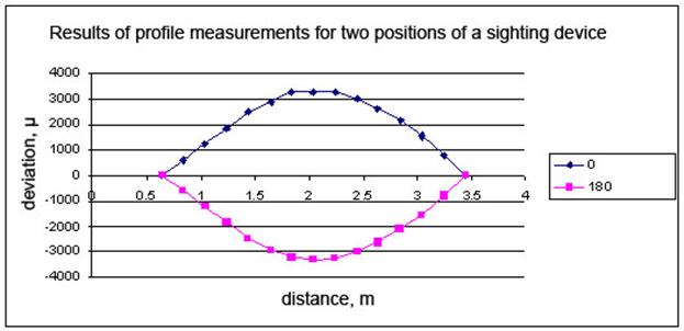
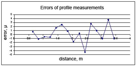
Graphs, constructed in Fig. 3, are useful in visualising the results of
profile measurements, relating to two abovementioned positions of a device, as
well as the error of measurements for each of the profile points, subject to
measurement. Said errors are estimated by determining the difference of results
of measurements, relating to two positions of a device. In both of the graphs,
constructed in Fig. 3, quantities of measurement distance in metres are plotted
on X-axis, while quantities of deviation from the base line in microns are
plotted on Y-axis of the upper graph, and error quantities in microns are
plotted on Y-axis of the lower graph. It may be seen that within the distance
range 0.7 – 3.5 metres the value of error does not exceed some microns.
As relating to the measurement process, described here, the basic
systematic error is the error of co-ordinates of the sighting line trace. If
distance values are great the basic systematic error practically has no
influence on the measurement process. That is why only those measurements,
which are performed at small distances, are of the greatest interest in the
field of metrology.
If one uses an optical device he must set a measurement cross hairs on a
device optical axis by way of alignment. And if one uses a digital meter,
presented here, he does not need to set a light sensitive matrix central point
on a device optical axis. It should be noted that setting a matrix central
point on a device optical axis is impossible due to the fact accuracy of
measurement of location of a measuring mark centre is as high as some fractions
of micron. Below is considered the simple method of determining co-ordinates of
a sighting line trace on a light sensitive matrix surface. This method includes
two runs of measurements of a component profile. When the first run of
measurements is performed digital device axis and sighting telescope axis
coincide, while during performing the second run of measurements a device is
swung relative to the sighting telescope axis by 180°. While making
calculations, relating to two versions of a component profile, the co-ordinates
of a sighting line trace remain common for each of the profile versions. The
summation with respect to all profile values is made (it should be noted that
the profile co-ordinates, relating to the abovementioned device positions, are
of opposite signs). Then one strives for minimisation of sum of the profile
values by way of selection the co-ordinates of the sighting line trace. This
procedure is executed without any difficulties by using the “Excel” program.
Calculated values of co-ordinates of the sighting line trace are entered into
the program database for the purpose of performing computations when the
digital meter is used.
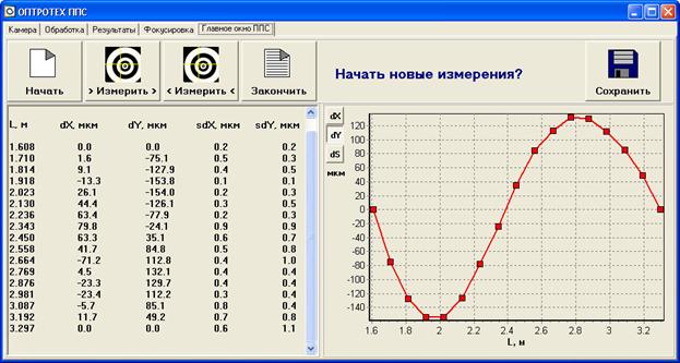
It should be pointed out that generating both the measurement protocol
and the graph of deviations of the mark centre from the base line is started by
the digital meter since the moment the measurement, relating to the third point
of the measurement route, is performed. The first point and the second point of
this route relate to the base line. Result of each of the subsequent
measurements is presented both in the protocol and the graph immediately.
Recalculation of data, relating to the base line, takes place any time a new
short-range or long-range end point appears. That is why while the measurement
cycle is being performed points may be arranged in any order. The final
measurement protocol and the graph, which presents a component profile, are
drawn up in the real-time mode, and drawing up of these documents finishes at
the moment the command “Complete” is generated. Generation of this command
takes place after the measurements, relating to the last one of the points,
have been performed (see Fig. 4).
Fig. 4
According to the instructions for use of the optical devices duration of
the process, needed to process the results of measurements, to calculate the
base line and to determine the profile deviations, is as long as 30 minutes. By
taking into account this fact anyone may become firmly convicted that capacity
of the digital meter is much greater than capacity of any optical device.
Reference list:
1. Anisimov A.G., Aleev A.M., Pantyushin A.V., Timofeev A.N., Basic errors of alignment control, revealed by using the automatic
reflection opto-electron system, “Optics Magazine”, volume 76, # 1, 2009, p.
3–8.
2. Pinaev L.V., Leontieva G.V., Butenko L.N., Seriogin A.G., Laser meter, used to determine error in linearity, Patent of the
Russian Federation # 2457434, 2010.
3. Apenko M.I., Araev V.A., Afanasiev V.A., Dureiko G.V., Zakaznov
N.P., Romanov D.A., Usov V.S., Optical devices,
used in the field of machine manufacturing, Reference Book, “Mashinostroenie”
Publishers, 1974, p. 120–167.
4. Danilevich F.M., Nikitin V.A., Smirnova E.P., Assembly and alignment of optical instrumentation, “Mashinostroenie”
Publishers, 1976, p. 222– 241.
5. Prospectus of the “Taylor
Hobson” company (www.taylor-hobson.com)
6. Koroliov A.N., Lukin A.Ya., Malinin S.M., Polishchuk G.S., Tregub
V.P., Digital meter, used to determine errors in
linearity and alignment, Patent of the Russian Federation # 112396, 2012.
|